
source(here::here("R/functions.R"))In [1]:
Introduction
THe correlation between physical activity, small vessel disease and classical risk factors is very much debated and not fully understood.(Moniruzzaman et al. 2020; Torres et al. 2019; Landman et al. 2021)
In this abstract, we present the preliminary results from our pooled SVD study, also presented at ESOC 2024.
Methods
This study is a cross-sectional study, based on a pooled dataset from two different randomised, clinical trials on patients with acute stroke.
Results
Please refer to Figure 1 for an overview of subjects included for analysis.
In [2]:
In [3]:
skimr::skim(targets::tar_read("complete_scores") |> (\(.i){
  .i |> dplyr::mutate(dplyr::across(names(.i)[-c(1:2)], ~ factor(.x)))
})())| Name | (function(.i) { |
| dplyr… | |
| Number of rows | 1055 |
| Number of columns | 12 |
| _______________________ | |
| Column type frequency: | |
| character | 2 |
| factor | 10 |
| ________________________ | |
| Group variables | None |
Variable type: character
| skim_variable | n_missing | complete_rate | min | max | empty | n_unique | whitespace |
|---|---|---|---|---|---|---|---|
| record_id | 0 | 1.00 | 5 | 8 | 0 | 1055 | 0 |
| user | 172 | 0.84 | 6 | 8 | 0 | 7 | 0 |
Variable type: factor
| skim_variable | n_missing | complete_rate | ordered | n_unique | top_counts |
|---|---|---|---|---|---|
| microbleed | 173 | 0.84 | FALSE | 5 | 0: 707, 1: 82, 2-4: 59, >10: 19 |
| siderose | 173 | 0.84 | FALSE | 3 | No : 877, 1 s: 4, > 1: 1 |
| lacunes | 173 | 0.84 | FALSE | 5 | 0: 614, 1: 122, 2: 70, 3-5: 61 |
| wmh | 174 | 0.84 | FALSE | 4 | 1: : 473, 2: : 193, 0: : 127, 3: : 88 |
| atrophy | 173 | 0.84 | FALSE | 4 | 1: : 321, 0: : 311, 2: : 226, 3: : 24 |
| microbleed_location___1 | 172 | 0.84 | FALSE | 2 | Unc: 785, Che: 98 |
| microbleed_location___2 | 172 | 0.84 | FALSE | 2 | Unc: 804, Che: 79 |
| microbleed_location___3 | 172 | 0.84 | FALSE | 2 | Unc: 832, Che: 51 |
| consensus | 172 | 0.84 | FALSE | 3 | dis: 379, agr: 254, con: 250 |
| svd_missing_reason | 883 | 0.16 | FALSE | 2 | Man: 169, And: 3 |
Skimmed overview of SVD scoring
Baseline characteristics are included with the Table 2.
In [4]:
In [5]:
targets::tar_read("complete_scores") |>
  dplyr::select(-c("record_id", "user")) |>
  dplyr::mutate(dplyr::across(
    dplyr::all_of(c("microbleed", "lacunes")),
    ~ factor(.x,
      levels = .x |>
        dsub("^>", "9r_") |>
        as.factor() |>
        levels() |>
        dsub("^9r_", ">")
    )
  )) |>
gtsummary::tbl_summary()In [6]:
targets::tar_read("clin_data") |>
  dplyr::select(-record_id, -trial_id, -inclusion_date) |>
gtsummary::tbl_summary(by = trial)| Characteristic | RESIST, N = 5461 | TALOS, N = 5091 |
|---|---|---|
| active_treatment | 256 (47%) | 251 (49%) |
| age | 74 (63, 80) | 70 (61, 78) |
| female_sex | 199 (36%) | 185 (36%) |
| pase_0 | 91 (55, 127) | 121 (65, 191) |
| Unknown | 128 | 0 |
| smoker | 120 (22%) | 160 (32%) |
| Unknown | 0 | 10 |
| alc_more | 60 (11%) | 49 (9.8%) |
| Unknown | 19 | 10 |
| alone | 148 (27%) | 160 (32%) |
| Unknown | 5 | 4 |
| diabetes | 68 (12%) | 54 (11%) |
| Unknown | 0 | 4 |
| hyperten | 329 (60%) | 262 (52%) |
| Unknown | 0 | 3 |
| pad | 19 (3.5%) | 23 (4.6%) |
| Unknown | 7 | 8 |
| afib | 89 (16%) | 94 (19%) |
| Unknown | 0 | 4 |
| ami | 49 (9.0%) | 43 (8.5%) |
| Unknown | 0 | 5 |
| ais | 91 (17%) | 0 (0%) |
| Unknown | 1 | 0 |
| tci | 40 (7.4%) | 15 (3.0%) |
| Unknown | 4 | 7 |
| tpa | 352 (64%) | 201 (40%) |
| Unknown | 0 | 6 |
| evt | 111 (20%) | 41 (8.1%) |
| Unknown | 0 | 5 |
| any_perf | 399 (73%) | 209 (42%) |
| Unknown | 0 | 6 |
| nihss | 4.0 (2.0, 9.0) | 4.0 (2.0, 7.0) |
| Unknown | 2 | 13 |
| mrs_eos | ||
| 0 | 136 (25%) | 100 (23%) |
| 1 | 176 (32%) | 168 (39%) |
| 2 | 88 (16%) | 114 (26%) |
| 3 | 80 (15%) | 29 (6.7%) |
| 4 | 19 (3.5%) | 21 (4.8%) |
| 5 | 14 (2.6%) | 3 (0.7%) |
| 6 | 33 (6.0%) | 0 (0%) |
| Unknown | 0 | 74 |
| pase_0_high | 170 (41%) | 293 (58%) |
| Unknown | 128 | 0 |
| 1 n (%); Median (IQR) | ||
In [7]:
In [8]:
targets::tar_read("df_complete") |>
  dplyr::filter(!is.na(pase_0), !is.na(simple_score)) |>
  get_vars(c("pre", "clin")) |>
  # dplyr::mutate(female_sex = dplyr::if_else(female_sex, "Female", "Male")) |>
  dplyr::transmute(simple_score, age, female_sex= dplyr::if_else(female_sex, "Female", "Male"), nihss, tpa, evt, pase_0, alone) |>
  labelling_data() |>
  gtsummary::tbl_summary(by = female_sex, missing = "no") |>
  # gtsummary::add_p() |>
gtsummary::add_overall()| Characteristic | Overall, N = 7651 | Female, N = 2801 | Male, N = 4851 |
|---|---|---|---|
| SVD score | |||
| 0 | 302 (39%) | 105 (38%) | 197 (41%) |
| 1 | 216 (28%) | 75 (27%) | 141 (29%) |
| 2 | 142 (19%) | 61 (22%) | 81 (17%) |
| 3 | 71 (9.3%) | 29 (10%) | 42 (8.7%) |
| 4 | 34 (4.4%) | 10 (3.6%) | 24 (4.9%) |
| Age | 71 (62, 79) | 75 (64, 80) | 70 (61, 77) |
| Admission NIHSS | 4.0 (2.0, 7.0) | 4.0 (2.0, 8.0) | 3.0 (2.0, 7.0) |
| Treated with tPA | 460 (60%) | 159 (57%) | 301 (62%) |
| Treated with EVT | 100 (13%) | 30 (11%) | 70 (14%) |
| Pre-stroke PASE score | 108 (60, 161) | 89 (55, 136) | 116 (71, 175) |
| Living alone | 203 (27%) | 120 (43%) | 83 (17%) |
| 1 n (%); Median (IQR) | |||
Scoring reliability between raters has been compared using different metrics, to show different nuances to the performance, see Table 3. The main performance measure is the intraclass correlation ceofficient.
In [9]:
targets::tar_read("ls_data") |>
  purrr::pluck("svd_score") |>
  dplyr::filter(svd_perf == "Ja", redcap_repeat_instance %in% 1:2) |>
  dplyr::select(record_id, redcap_repeat_instance, svd_microbleed, svd_lacunes, svd_wmh, svd_atrophy) |>
  simple_score() |>
  tibble::as_tibble() |>
  irr_icc_calc() |>
  gt::gt() |>
  gt::fmt_number(n_sigfig = 2)
Warning: Using an external vector in selections was deprecated in tidyselect 1.1.0.
ℹ Please use `all_of()` or `any_of()` instead.
# Was:
data %>% select(.x)
# Now:
data %>% select(all_of(.x))
See <https://tidyselect.r-lib.org/reference/faq-external-vector.html>.Joining with `by = join_by(Variable)`In [10]:
| Variable | Agreement | Krippendorffs_Alpha | Fleiss_Kappa | Brennan_Predigers_Kappa | IntraclCorrCoef |
|---|---|---|---|---|---|
| microbleed | 0.90 | 0.65 | 0.65 | 0.80 | 0.65 |
| lacunes | 0.83 | 0.56 | 0.56 | 0.66 | 0.56 |
| wmh | 0.88 | 0.72 | 0.72 | 0.75 | 0.72 |
| atrophy | 0.81 | 0.54 | 0.54 | 0.63 | 0.54 |
| score | 0.62 | 0.46 | 0.46 | 0.52 | 0.75 |
Below is the initial evaluation of possible PA effect modification on classical risk factors, Table 4. These results indicates no effect modification as odds ratios are largely unchanged, when PA is introduced in the model (on the right). This may not be the optimal method for this kind of evaluation, though.
In [11]:
In [12]:
ls <- c(FALSE, TRUE) |>
  purrr::map(main_analysis, get_vars(targets::tar_read("df_complete"), vars.groups = "poster") |>
    dplyr::mutate(
      simple_score = factor(simple_score)
    )) |>
  purrr::map(function(.x) fix_labels(.x)) |>
  setNames(c("1 Without PA", "2 With PA"))

p1 <- ls |>
  purrr::imap(function(.x, .i) {
    .x[["table_body"]] |>
      dplyr::select(label, estimate, conf.low, conf.high) |>
      dplyr::mutate(model = .i)
  }) |>
  dplyr::bind_rows() |>
  dplyr::mutate(
    label = factor(label, levels = rev(get_set_label("poster")[-1]))
  ) |>
  coef_forrest_plot(cols = viridis::viridis(7)[c(1,5)] )

p1 + ggplot2::facet_wrap(facets = ggplot2::vars(model), ncol = 2)
# p1 |> poster_coef_print(here::here("post.png"))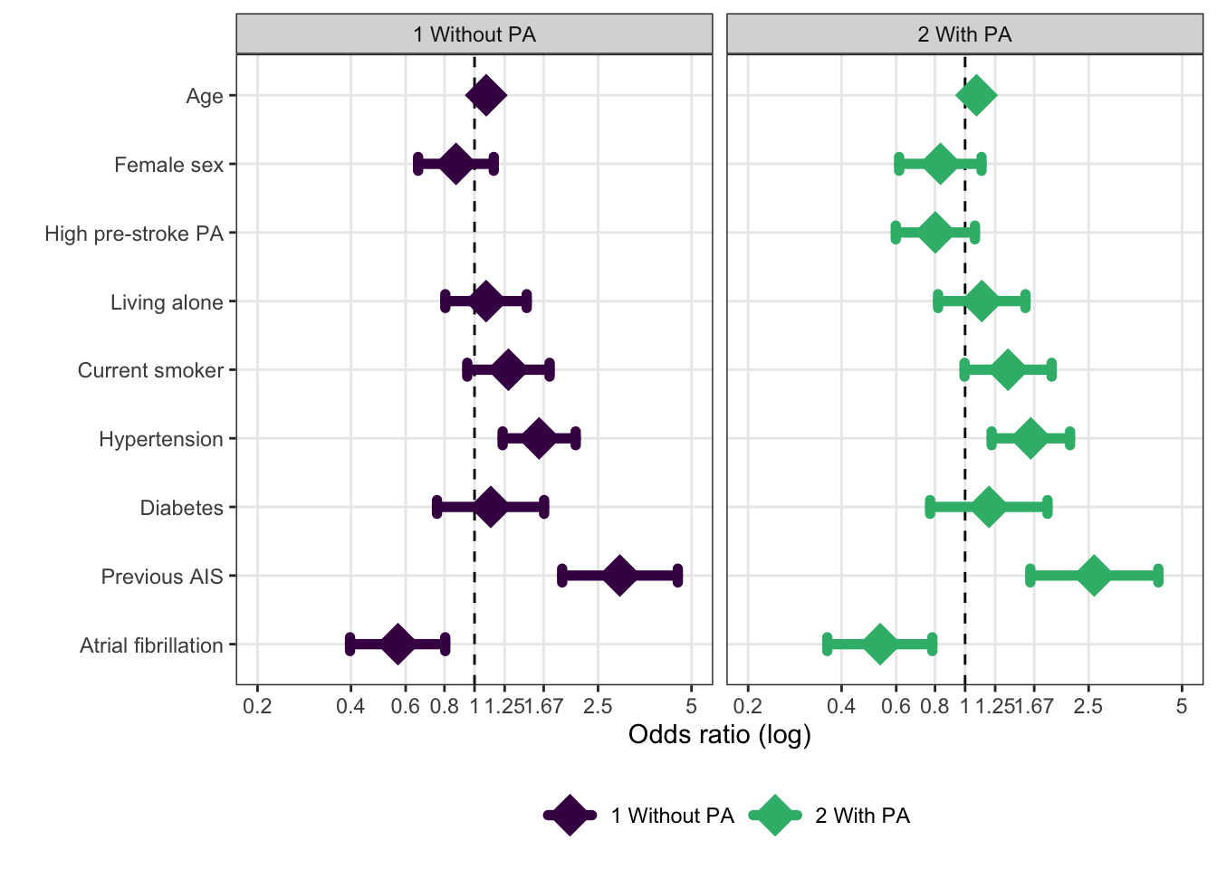
In [13]:
p <- targets::tar_read("df_complete") |>
  dplyr::transmute(simple_score,
    hyperten = dplyr::if_else(hyperten, "Hypertension", "No hypertension"),
    pase_0 = stRoke::quantile_cut(pase_0, groups = 2, group.names = c("Low PA level", "High PA level"))
  ) |>
  table() |>
  rankinPlot::grottaBar(
    scoreName = "simple_score",
    groupName = "hyperten",
    strataName = "pase_0",
    textColor = c("black", "white"),
    textCut = 3,
    printNumbers = "count"
  ) +
  ggplot2::labs(fill = "SVD score") +
  viridis::scale_fill_viridis(discrete = TRUE, direction = -1, option = "viridis")
Scale for fill is already present.
Adding another scale for fill, which will replace the existing scale.p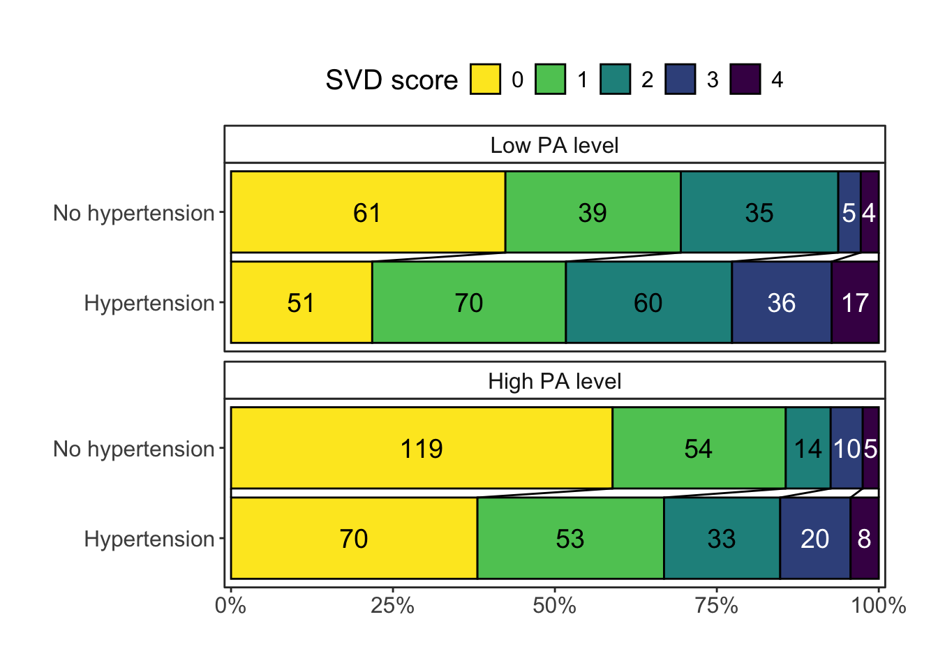
Based on the preliminary SVD-scores, SVD score distribution stratified by PA quartile is presented in Figure 2.
In [14]:
# renv::install("agdamsbo/rankinPlot")
p <- targets::tar_read("df_complete") |>
  dplyr::transmute(simple_score,
    pase_0 = stRoke::quantile_cut(pase_0,
      groups = 4,
      group.names = glue::glue("Q{1:4}")
    )
  ) |>
  table() |>
  rankinPlot::grottaBar(
    scoreName = "simple_score",
    groupName = "pase_0",
    textColor = c("black", "white"),
    textCut = 3,
    printNumbers = "none",
    lineColor = "black",
    lineSize = 1,
    drawLines = FALSE,
    returnData = TRUE
  ) |>
  (\(.x){
    .x$plot + ggplot2::geom_text(data = .x$rectData[which(.x$rectData$n >
  0), ],
  # size = 6,
  fontface = "plain", ggplot2::aes(
  x = group,
  y = p_prev + 0.49 * p, color = as.numeric(score) >
    2,
  # label = paste0(sprintf("%2.0f", 100 * p),"%"),
  label = paste0(sprintf("%2.0f", 100 * p), "%")
)) +
  ggplot2::labs(fill = "SVD score") +
  ggplot2::ylab("Physical activity level")+
  viridis::scale_fill_viridis(discrete = TRUE, direction = -1, option = "D")
  })()
Scale for fill is already present.
Adding another scale for fill, which will replace the existing scale.p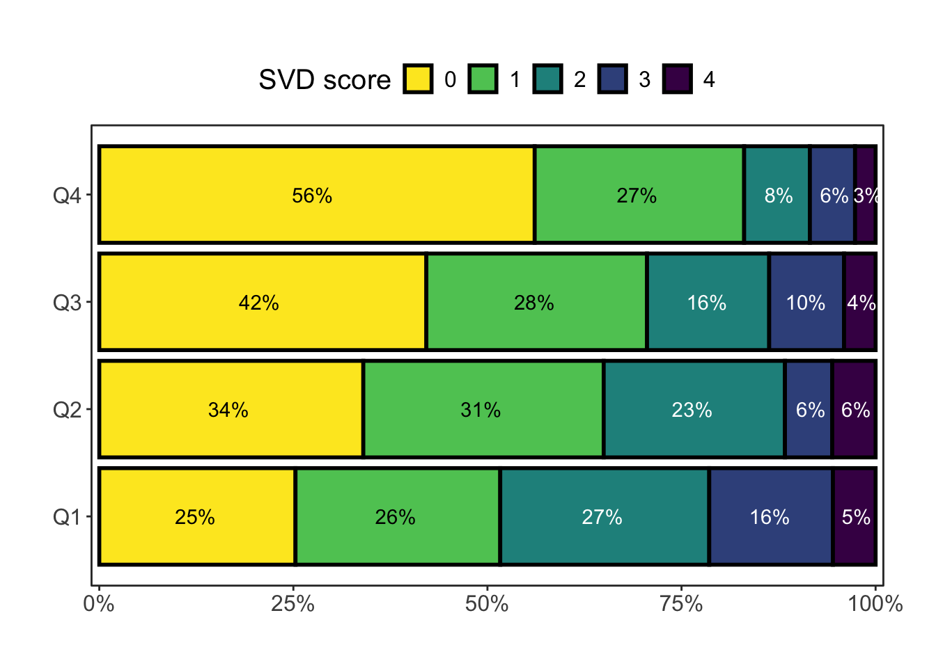
In [15]:
ggplot2::ggsave(
  filename = here::here("grotta_pa_svd.png"),
  p +
    ggplot2::theme_minimal() +
    ggplot2::theme(
      legend.position = "none",
      panel.grid.major = ggplot2::element_blank(),
      panel.grid.minor = ggplot2::element_blank(),
      panel.border = ggplot2::element_blank(),
      panel.grid = ggplot2::element_blank(),
      axis.text.y = ggplot2::element_blank(),
      axis.title.y = ggplot2::element_blank(),
      axis.text.x = ggplot2::element_blank(),
      axis.title.x = ggplot2::element_blank(),
      text = ggplot2::element_text(size = 25),
      plot.title = ggplot2::element_text(),
      panel.background = ggplot2::element_blank()
    ),
  units = "cm",
  width = 65,
  height = 12,
)
In [16]:
targets::tar_read("df_complete") |>
  get_vars(vars.groups = c("pre")) |>
  (\(ds){
    genodds::genodds(response = ds$simple_score, group = stRoke::quantile_cut(ds$pase_0, groups = 2, group.names = c("low", "high")), strata = ds$diabetes)
  })()
Warning in genodds::genodds(response = ds$simple_score, group =
stRoke::quantile_cut(ds$pase_0, : Dropped 291 observations with missing values Agresti's Generalized odds ratios
FALSE Odds: 0.618 (0.521, 0.733) p=0.0000
TRUE Odds: 0.678 (0.420, 1.093) p=0.1109
Test of H0: odds ratios are equal among strata:
X-squared = 0.13, df= 1 p=0.7209
Test of H0: pooled odds = 1:
Pooled odds: 0.624 (0.532,0.733) p=0.0000
--------------------------------------------
In the FALSE stratum:
Of 100 patients given high instead of low:
* 24.81 will score higher with high
* 48.43 will score higher with low
* 26.76 appear the same with either treatment
In the TRUE stratum:
Of 100 patients given high instead of low:
* 27.62 will score higher with high
* 46.83 will score higher with low
* 25.55 appear the same with either treatmenttargets::tar_read("df_complete") |>
get_vars(vars.groups = c("pre","post")) |>
(\(ds){
genodds::genodds(response = ds$mrs_eos, group = ds$simple_score == 0, strata = ds$active_treatment)
})()Warning: Unknown or uninitialised column: `active_treatment`.Warning in genodds::genodds(response = ds$mrs_eos, group = ds$simple_score == :
Dropped 225 observations with missing values Agresti's Generalized odds ratios
Odds: 0.759 (0.651, 0.884) p=0.0004
--------------------------------------------
Of 100 patients given TRUE instead of FALSE:
* 30.77 will score higher with TRUE
* 44.51 will score higher with FALSE
* 24.72 appear the same with either treatmentDiscussion
The numbers and figures presented here are very much preliminary and should only be used for discussion and inspiration. Also, if you have any interest in collaboration, please reach out!
Landman, Thijs Rj, Dick Hj Thijssen, Anil M. Tuladhar, and Frank-Erik de Leeuw. 2021. “Relation between physical activity and cerebral small vessel disease: A nine-year prospective cohort study.” International Journal of Stroke: Official Journal of the International Stroke Society 16 (8): 962–71. https://doi.org/10.1177/1747493020984090.
Moniruzzaman, Mohammad, Aya Kadota, Hiroyoshi Segawa, Keiko Kondo, Sayuki Torii, Naoko Miyagawa, Akira Fujiyoshi, et al. 2020. “Relationship Between Step Counts and Cerebral Small Vessel Disease in Japanese Men.” Stroke 51 (12): 3584–91. https://doi.org/10.1161/STROKEAHA.120.030141.
Torres, Elisa R., Siobhan M. Hoscheidt, Barbara B. Bendlin, Vincent A. Magnotta, Gabriel D. Lancaster, Roger L. Brown, and Sergio Paradiso. 2019. “Lifetime Physical Activity and White Matter Hyperintensities in Cognitively-Intact Adults.” Nursing Research 68 (3): 210–17. https://doi.org/10.1097/NNR.0000000000000341.