Beautiful sankey plot

Usage

plot_sankey_single(
  data,
  pri,
  sec,
  color.group = c("pri", "sec"),
  color.palette = "viridis",
  colors = NULL,
  missing.level = "Missing",
  default.color = "#2986cc",
  box.color = "#1E4B66",
  na.color = "grey80",
  ...
)

Arguments

color.group: set group to colour by. "x" or "y".
colors: optinally specify colors. Give NA color, color for each level in primary group and color for each level in secondary group.
...: passed to sankey_ready()

Value

ggplot2 object

Examples

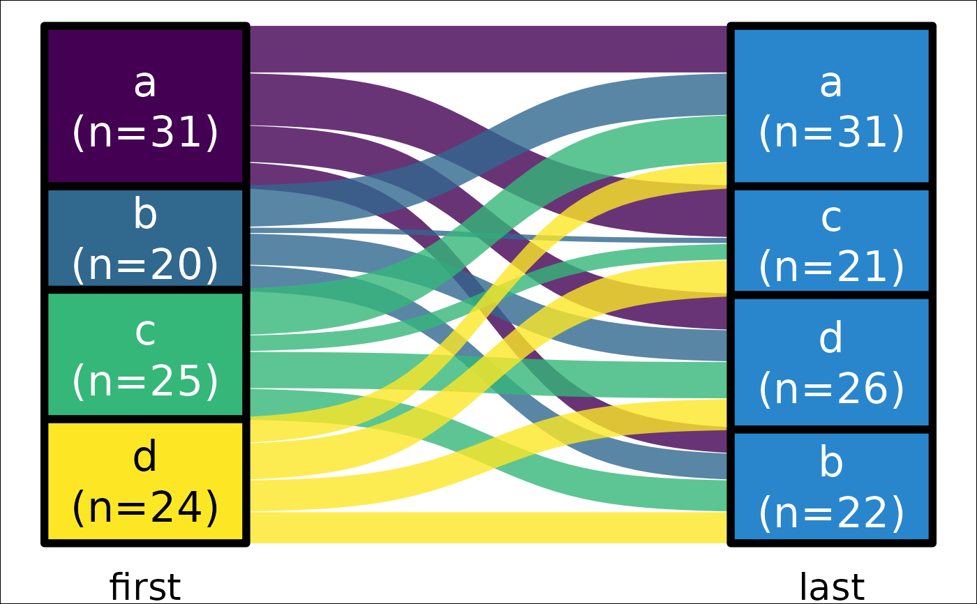
ds <- data.frame(g = sample(LETTERS[1:2], 100, TRUE), first = REDCapCAST::as_factor(sample(letters[1:4], 100, TRUE)), last = REDCapCAST::as_factor(sample(letters[1:4], 100, TRUE)))
ds |> plot_sankey_single("first", "last")

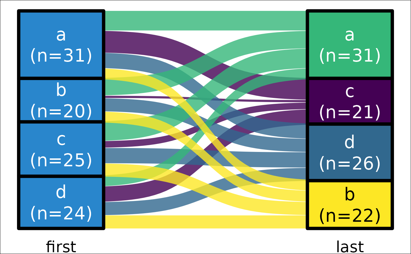
ds |> plot_sankey_single("first", "last", color.group = "sec")

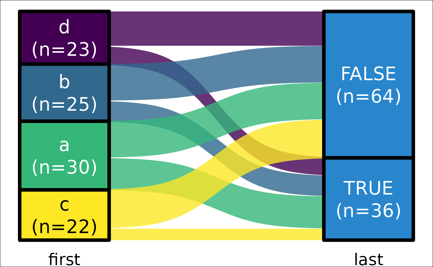
data.frame(
  g = sample(LETTERS[1:2], 100, TRUE),
  first = REDCapCAST::as_factor(sample(letters[1:4], 100, TRUE)),
  last = sample(c(TRUE, FALSE, FALSE), 100, TRUE)
) |>
  plot_sankey_single("first", "last", color.group = "pri")

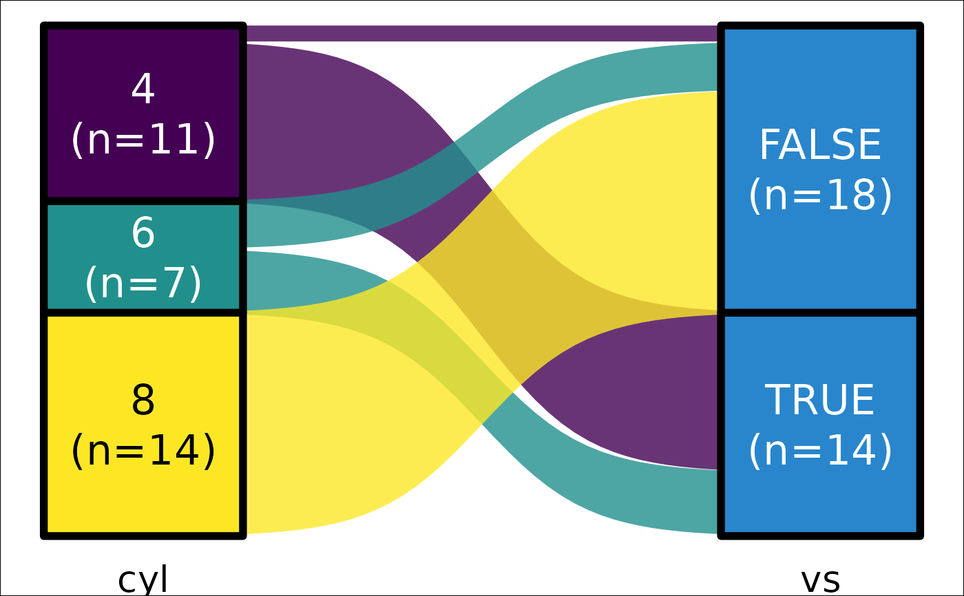
mtcars |>
  default_parsing() |>
  plot_sankey_single("cyl", "vs", color.group = "pri")

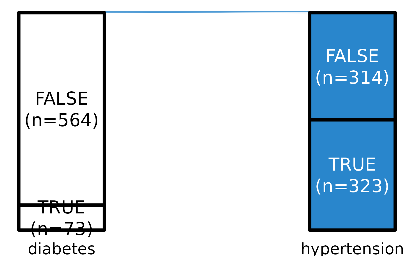
stRoke::trial |>
  default_parsing() |>
  plot_sankey_single("diabetes", "hypertension")
#> Warning: Some strata appear at multiple axes.
#> Warning: Some strata appear at multiple axes.
#> Warning: Some strata appear at multiple axes.



 # stRoke::trial |> plot_sankey_single("mrs_1", "mrs_6", color.palette="magma")
 # stRoke::trial |> plot_sankey_single("active", "male")
 # stRoke::trial |> plot_sankey_single("diabetes", "active", color.group="sec")
 # stRoke::trial |> plot_sankey_single("active", "diabetes", color.group="sec", color.palette="topo")