6 ZIP to data set

Authors

Affiliations

Christina Rubino

So, here I’ll show how we went from compressed zip file, from the NeMo tool, and to having a data set for further analyses.

I am fairly new to Python, but have worked in R for many years. This means, that I have written just enough in Python, and everything else in R. Small python functions will be wrapped in R scripts. Just a word of warning.

First, extract the compressed file and put it where you like. I’ll denote this location as the source.folder.

# source.folder <- "/full/path/NeMo_output"
source.folder <- "/Users/au301842/NeMo_output"

Then we want to extract the chacovol data. This is extracted by unpikling .pkl files using a short python script wrapped in R:

source("nemo/unpkl-sparse.R")
unpkl_sparse(data.folder = source.folder,
             "chacovol_yeo17_mean.pkl")

The unpikled files are then collected and merged in a wide format.

But first, we need to handle the provided atlas .txt files to get ROI names:

atlas <- readLines("/Users/au301842/NeMo_output/Yeo2011_17Networks_NetworkNames_ColorLUT.txt")
rois <- do.call(c,lapply(atlas[-1],function(i){
  s1 <- strsplit(i,"_[0-9]{1,3}_")[[1]][2]
  strsplit(s1," ")[[1]][1]
  }
  ))

source("nemo/nemo-collect.R")
df <- nemo_collect(
  data.folder = source.folder,
  id.pattern = "W[0-9]{2}",
  file.pattern = "chacovol_yeo17_mean.tsv",
  roi.names = rois
)

I very much prefer writing function to do the data handling, but I just have to note, that these functions are very primitive due to lack of time on my end. But they are working and will provide a good foundation for further worker.

6.1 Visualisation

Please note that the NeMo-repository is shared without a license

This means it is technically not allowed to modify or redistribute the code. Please refer to {#contents}.

We also want those nice glass brains. These following R scripts are all simple wrappers for the scripts from the NeMo tool, which uses the nibabel Python package for plotting. All the examples below are created based on a small sample of two subjects and the Yeo17 atlas which is also shared in the NeMo tool source.

First we do the simpel voxel based heatmap.

source("nemo/glass-brain.R")
glass_brain(
  data.folder = source.folder,
  file.pattern = "chacovol_res2mm_mean.nii.gz",
  out.name = "images/glass_chacovol.png"
)

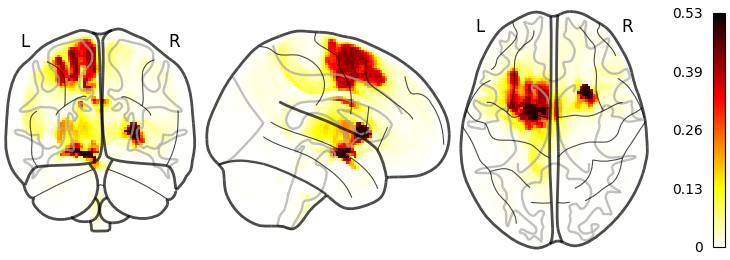Averaged voxel based chacovol glassbrain plot Next we can do the parcellation or atlas based chacovol plotting:

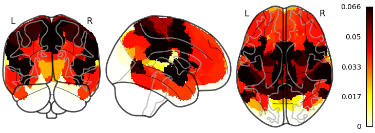
source("nemo/glass-brain.R")
glass_brain(
  data.folder = source.folder,
  file.pattern = "chacovol_yeo17_mean.pkl",
  out.name = "images/glass_chacovol_parc.png",
  parcellation = "/Users/atlas/folder/Yeo2011_17Networks_MNI152_182x218x182_LiberalMask.nii.gz"
)

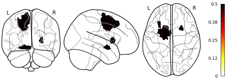
Averaged parcellation based chacovol glassbrain plot

The same scirpt can also be used for lesion plotting:

glass_brain(
  data.folder = "/Users/folder/with/lesions/",
  file.pattern = "lesion.nii.gz",
  id.pattern = "W(50|49)", # This id.pattern is used to only include specified ids
  out.name = "images/glass_lesion.png"
)

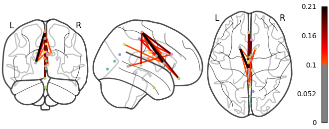
And finally the change in connections between areas in the brain can be visualised as a graphbrain:

source("nemo/graph-brain.R")
graph_brain(
  data.folder = source.folder,
  file.pattern = "chacoconn_yeo17_mean.pkl",
  out.name = "images/glass_chacoconn.png",
  node.file="/Users/atlas/folder/Yeo2011_17Networks_MNI152_182x218x182_LiberalMask.nii.gz"
)

Graph brain plot of lost connections between atlas based ROIs

6.2 Glossary

data frame with 0 columns and 0 rows